An IC50 fit can fail visibly, with an optimizer error, or quietly, with a precise-looking number that the experiment does not support. Before changing fitting settings, check three things: the definition of IC50, the concentration range, and the way the response was normalized.
This guide uses a simulated inhibition dataset to separate those problems. The supplied CSV, fitted values, and figure come from an independent Python calculation. No compound was tested, and these are not results from a Gradiance run.
1. Decide which 50% you mean
A relative IC50 is the concentration halfway between the fitted upper and lower response plateaus. An absolute IC50 is the concentration at the assay’s 50%-of-control response. Sebaugh’s estimation guidelines distinguish these definitions and describe the data needed to support each. [1]
Consider a descending curve whose top is 100% activity and whose bottom is 20%. Its relative midpoint is at 60% activity, halfway between those plateaus. Reaching 50% of the control activity requires a higher concentration. Both can be meaningful endpoints, but they are not interchangeable.
Activity(x) = Bottom + (Top − Bottom) / [1 + (x / C)^H]

Relative midpoint: C
Absolute 50% crossing:
x50 = C × [(Top − Bottom) / (50 − Bottom) − 1]^(1/H)
That crossing formula assumes a descending curve with positive slope parameter H and Bottom < 50 < Top. If the fitted bottom is above 50%, the curve never reaches the absolute endpoint. Software should not turn that situation into an ordinary numerical IC50.
2. Check whether the tested range contains the answer
Our teaching dataset contains 11 log-spaced concentrations from 0.01 to 1,000 µM and three simulated observations per concentration. We generated it with Top = 100, Bottom = 20, C = 3 µM, and H = 1.2, then added normal noise with standard deviation 1.2 percentage points using seed 609.
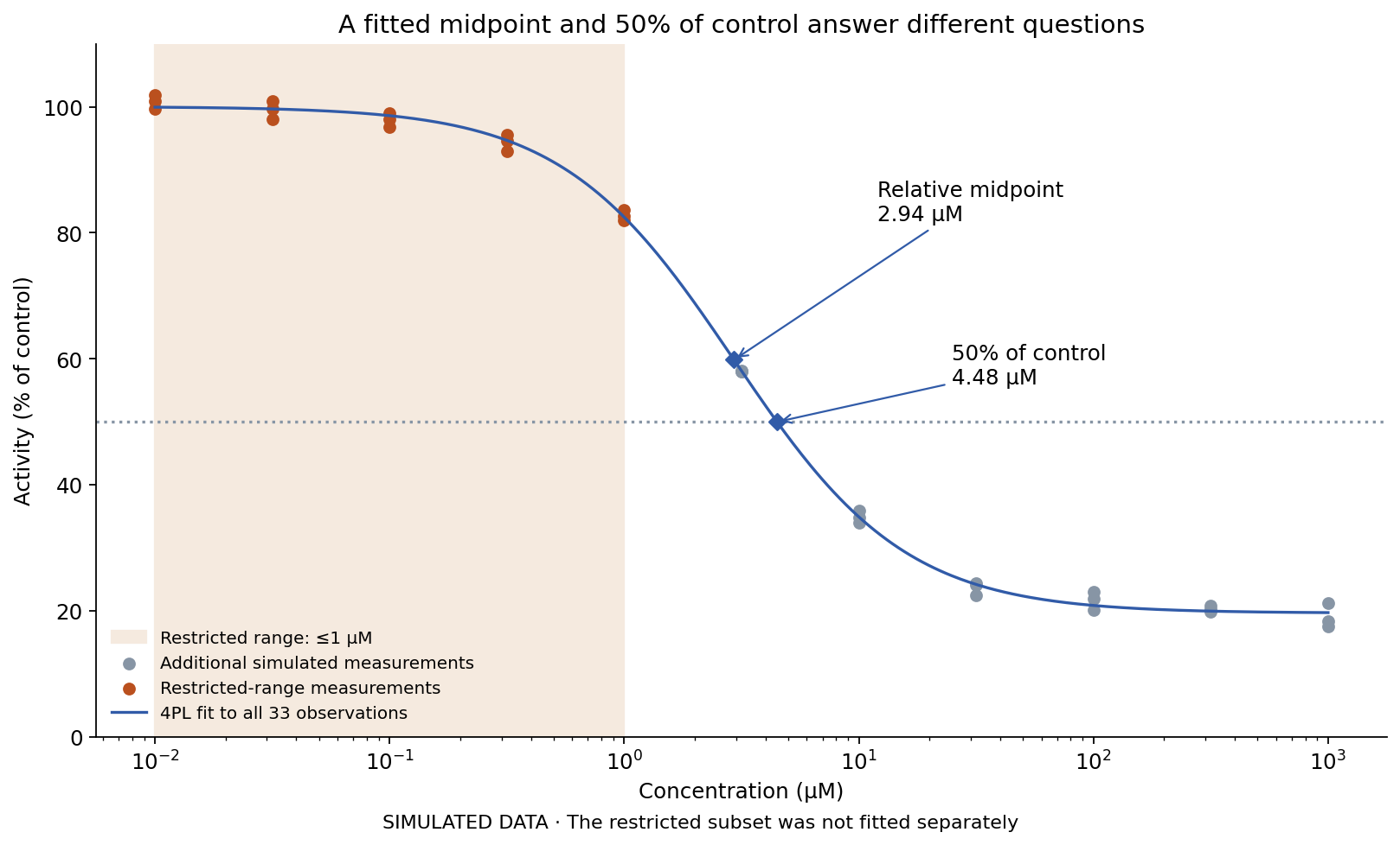
An unweighted fit to all observations gives a top of 100.04%, bottom of 19.66%, and slope of 1.183. The relative midpoint is 2.94 µM, while the 50%-of-control crossing is 4.48 µM. Those numbers differ because they answer different questions, not because one calculation failed.
Now retain only concentrations at or below 1 µM. The resulting 15 observations never fall below 82.05% activity. They contain neither a lower plateau nor an observed crossing of 50% activity. The complete-curve answer cannot be recovered from those points by simply requesting more decimal places.
For a real experiment like that restricted example, report that the absolute 50% endpoint was not reached over the tested range. A statement such as “IC50 >1 µM” needs the endpoint definition, assay QC, and reporting rules to support it. Extend the concentration range only within experimentally appropriate solubility, interference, and assay limits. This simulated subset is not evidence of biological inactivity.
3. Normalize against controls with a defined role
For an assay where signal increases with activity, one possible control-based calculation is:
Activity (%) = 100 × (sample − low control) / (vehicle − low control)
Inhibition (%) = 100 − Activity (%)
The low control must represent the intended low-activity reference for the assay; a reagent blank and a fully inhibited biological sample are not automatically equivalent. Record the control identities and how replicate control values are summarized. The Assay Guidance Manual discusses normalization with respect to positive and negative controls. [2]
Do not silently redefine the weakest response from each compound as 0% activity. In our example, rescaling a 20% plateau to zero would change which response counts as “50%.” Preserve the raw readings and control measurements so another analyst can reconstruct that choice.
4. Match the symptom to the next check
| Symptom | Inspect first | Useful next step |
|---|---|---|
| No convergence | Units, missing values, concentration encoding | Confirm whether the model expects concentration or log concentration; inspect starting values and bounds. |
| Huge or unstable IC50 | Coverage around both plateaus and the transition | Review uncertainty and whether the endpoint lies outside the tested range. |
| One well bends the curve | Raw signal, plate location, replicate agreement | Investigate the well and compare an explicitly documented sensitivity fit. |
| A parameter hits its bound | The rationale for that bound | Check whether the constraint is replacing missing information. |
| Response falls, then rises | Plate effects, solubility, interference, mixed responses | Investigate the assay; a monotonic 4PL or 5PL cannot represent a genuinely biphasic response. |
Plot individual observations and residuals before excluding anything. Keep the original analysis, state the reason for any exclusion, and show how it affects the endpoint. The Assay Guidance Manual explains that an outlier’s position can affect different curve parameters. Removing a point because the fit improves is not an independent explanation for its exclusion. [2]
Similarly, fixing the bottom at zero needs experimental justification. In our simulated dataset the generating bottom is 20%, so a zero-bottom constraint contradicts the example by construction. A different optimizer cannot resolve that mismatch. Review model assumptions before treating convergence as evidence of a sound analysis.
5. Report enough context to interpret the number
Include the endpoint definition, concentration units and range, model equation, free and fixed parameters, normalization controls, weighting, exclusions, and uncertainty method. Separate replicate wells from independent experiments. The 33 observations in this illustration are simulated measurements, not 33 biological replicates. We report point estimates to demonstrate the endpoint distinction; we have not calculated confidence intervals here.
When preparing an analysis in Gradiance, use the dose-response guide and quality-control reference. State the intended endpoint in the request and inspect the returned equation and parameters. For asymmetric calibration curves, see the companion 4PL versus 5PL worked example.
Reproduce the example
- Simulated concentrations and activity values (CSV)
- Python script for all three teaching examples
- Calculated results and package versions
Install NumPy, SciPy, and Matplotlib in a Python environment, then run python reproduce.py --output generated. The script generates the simulated data, performs the calculations, and draws the figures locally. It does not call Gradiance or submit data to a service. Our recorded versions are NumPy 1.26.4, SciPy 1.17.1, and Matplotlib 3.10.9.
References
- Sebaugh JL. Guidelines for accurate EC50/IC50 estimation. Pharmaceutical Statistics. 2011;10(2):128–134. DOI: 10.1002/pst.426.
- Beck B et al. Assay Operations for SAR Support. Assay Guidance Manual. NCBI Bookshelf.