A standard curve can look convincing while giving biased concentrations for your unknowns. Choosing between a four-parameter logistic model (4PL) and a five-parameter logistic model (5PL) means checking what happens when you invert the curve, as well as how closely it follows the standards.
Start with the model specified by your assay protocol. When developing a method, a 4PL is a useful baseline; evaluate a 5PL if reproducible asymmetry remains after checking preparation, weighting, and measurement problems. The fifth parameter adds flexibility, which also makes it another quantity your data must support.
About this example: the data and plots below are simulated, with a known asymmetric generating curve. They illustrate a model-choice problem. They are not measurements from an ELISA kit, a Gradiance run, or a product benchmark.
What changes between 4PL and 5PL?
For an increasing calibration curve, we use this parameterization with positive concentrations:
y = B + (T − B) / [1 + (C / x)^H]^S

B: lower plateau       T: upper plateau
C: concentration scale H: positive slope parameter
S: asymmetry parameter; fixing S = 1 gives a 4PL
The 4PL is symmetric around its midpoint on a log-concentration axis. Allowing S to vary changes that symmetry. Gottschalk and Dunn describe how the additional parameter can improve concentration estimation for asymmetric assays, while also discussing designs that make fitting difficult. Their result supports evaluating asymmetry; it does not establish that every assay needs a 5PL. [1]
Parameter names differ across software. In the equation above, setting x = C gives B + (T − B) / 2^S. That is halfway between the plateaus only when S = 1. The actual halfway concentration is:
x50 = C / (2^(1/S) − 1)^(1/H)For the generating values in this example, C = 4, H = 1.1, and S = 0.45. Calling the scale parameter an EC50 without checking the equation would therefore change the meaning of the reported result.
A worked comparison with known concentrations
We generated 12 logarithmically spaced concentrations from 0.01 to 1,000 arbitrary units, with three simulated observations at each level. The true plateaus are 0.08 and 2.40 signal units. Independent normal noise with standard deviation 0.015 is added to each observation, using random seed 608.
Both fits use all 36 observations and unweighted nonlinear least squares. Equal weighting matches this example’s constant noise variance. The script fits positive parameters in log coordinates, tries multiple starting values, and selects the converged solution with the smallest residual sum of squares. Bounds and initial values are included in the download.
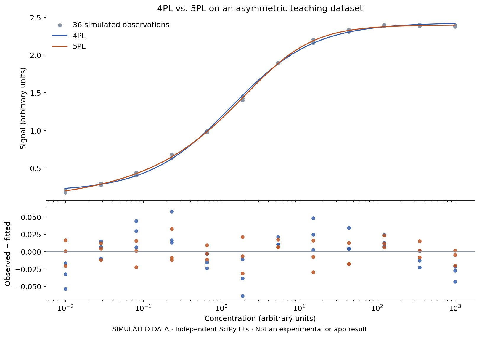
The residual root mean square error is 0.02747 for 4PL and 0.01543 for 5PL. A smaller residual alone is insufficient to justify the extra parameter. To examine the consequence for quantification, we generated noiseless signals at three additional known concentrations and inverted each fitted curve:
| Known concentration | 4PL estimate | 4PL error | 5PL estimate | 5PL error |
|---|---|---|---|---|
| 0.10 | 0.1110 | +11.0% | 0.0936 | −6.4% |
| 1.00 | 0.9350 | −6.5% | 0.9922 | −0.8% |
| 10.00 | 11.3230 | +13.2% | 10.1448 | +1.4% |
The 5PL reduces absolute error at these three locations in this example. We deliberately generated an asymmetric 5PL curve, so that outcome is unsurprising. The check signals are mathematical reference values, not independent laboratory QC samples. This one seed does not estimate how often either model wins across experiments.
How to choose for your assay
- Inspect the original measurements. Plot individual replicate wells. Check dilution labels, units, blanks, and signs of saturation before changing the equation.
- Keep the comparison fair. Use the same standards, exclusions, and justified error model for both candidates. If noise grows with signal, assess an appropriate weighting model; changing weights and curve shape together obscures the reason for improvement.
- Look for a repeatable pattern. Examine residuals across multiple runs. A few scattered points or one failed standard are weak grounds for introducing asymmetry.
- Evaluate the intended output. For quantification, inspect back-calculated standards and independently prepared QCs throughout the intended range. Choose acceptance criteria before comparing results.
- Check stability. Review uncertainty, sensitivity to starting values, and parameters pressing against bounds. A fitted asymmetry parameter is not useful if small changes produce very different concentration estimates.
Near a flat plateau, a small signal error can translate into a large concentration error: locally, the inverse sensitivity is proportional to 1 / (dy/dx). Adding a parameter cannot create information where the signal barely changes. Keep unknowns within a range supported by your assay’s precision and recovery; dilute or remeasure samples when appropriate.
Also distinguish selecting a calibration model from validating an assay. This illustration supplies no acceptance limits, clinical claims, or evidence of cross-run reproducibility. For a practical starting point, record which model you chose, its equation and weights, the standards retained, and the QC results that supported the decision.
Reproduce the calculation
- Simulated standard concentrations and signals (CSV)
- Python script for all three teaching examples
- Calculated results and package versions
Install NumPy, SciPy, and Matplotlib in a Python environment, then run python reproduce.py --output generated. The script generates the simulated data, performs the calculations, and draws the figures locally. It does not call Gradiance or submit data to a service. Our recorded versions are NumPy 1.26.4, SciPy 1.17.1, and Matplotlib 3.10.9.
For the application workflow, see standard curves and quantification. If your main concern is an inhibitory curve with a missing plateau, continue with why an IC50 curve fit fails. The 4PL/5PL comparison here is performed by the downloadable script; it does not verify a particular model-selection workflow in the app.
Reference
[1] Gottschalk PG, Dunn JR. The five-parameter logistic: a characterization and comparison with the four-parameter logistic. Analytical Biochemistry. 2005;343(1):54–65. DOI: 10.1016/j.ab.2005.04.035.