In a Gradiance run on the open Puromycin dataset, four fitted parameter values agreed with an independent calculation to within 0.001%. The same run had missing unit labels, a lost original request after a failure, and progress updates that required a page reload.
Those observations belong in the same account. The parameter comparison answered a narrow numerical question. The workflow problems affected what a researcher could see, recover, and report. Checking an AI-generated lab analysis means following both.
The original run report preserves the details and the later corrections. Here we use it to work through a review that starts with the input and ends with the claim you intend to make.
Start with the experiment the software actually analyzed
Match the output to the uploaded file, relevant sheet, conditions, and observation counts. Then inspect the column mapping and units. A fit can be internally consistent after a concentration column has been assigned the wrong unit.
The R documentation describes Puromycin as 23 reaction-rate observations, with concentration in ppm and rate in counts/min/min. It has 12 treated and 11 untreated observations. The experiment was conducted once per condition. Those counts describe observations within the curves; they do not supply independent biological replication for a treatment comparison. [1]
Our numerical reference fits the conditions separately, retaining every observation. That scope is part of the result. Pooling the two conditions, averaging selected rows, or dropping a high residual would produce a different analysis even if the resulting figure looked tidy.
Look at what the curve leaves unexplained
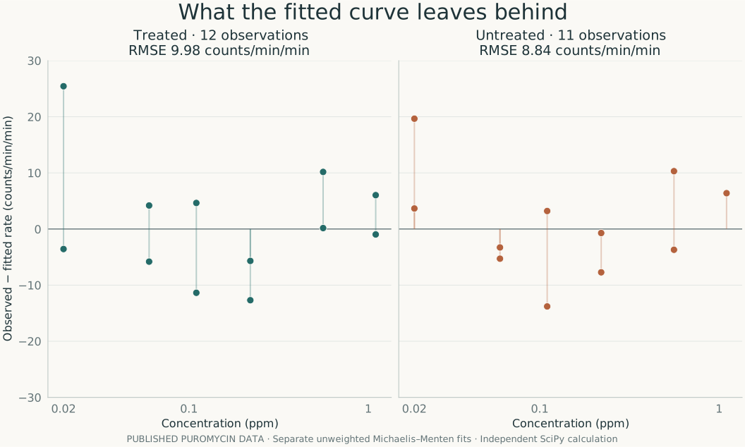
A residual is the observed response minus the fitted response. Plotting it makes departures from the fitted curve easier to inspect. The figure below was generated by refitting the published source data with an independent SciPy script. It is a new diagnostic figure, not a new Gradiance run.
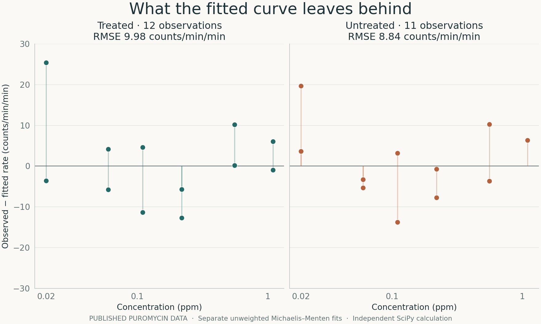
The residual RMSE is 9.98 counts/min/min for the treated curve and 8.84 counts/min/min for the untreated curve. You can also see observations at the same concentration falling on different sides of the fitted value. A single goodness-of-fit number compresses that information.
Use this view to ask specific questions. Are deviations concentrated at one end of the range? Does their spread change with concentration? Do repeated measurements disagree more than expected from the assay? Investigate those questions against the protocol and raw record before changing the fit.
Neither the plotted residuals nor the reported R² values establish a mechanism or a statistically significant treatment effect. They describe agreement between these observations and these fitted curves.
Repeat the calculation you intend to check
For a numerical comparison, start from the same input values and match the model equation, preprocessing, weights, constraints, and retained observations. Record the software versions and the tolerance used to compare results. Otherwise, a disagreement may reflect different methods rather than a software defect.
Our reference uses unweighted Michaelis–Menten fitting with nonnegative parameter bounds and initial values Vmax = 200 and Km = 0.05. It imports no Gradiance analysis code. Both the app calculation and the reference use SciPy, so this is an independent implementation of the check, not a comparison between different numerical libraries.
| Condition | Parameter | Live result | Reference |
|---|---|---|---|
| Treated | Vmax (counts/min/min) | 212.683859 | 212.683579 |
| Treated | Km (ppm) | 0.06412146 | 0.06412103 |
| Untreated | Vmax (counts/min/min) | 160.280124 | 160.280153 |
| Untreated | Km (ppm) | 0.04770830 | 0.04770835 |
The units in this table come from the dataset documentation; the historical live output omitted them. Agreement of these four point estimates does not validate the reported confidence intervals, establish their coverage, or test the full product. Each of those would require its own evidence.
Check what an export can reproduce
Open a downloaded script and identify its inputs. A file that redraws a curve from saved parameters can be useful for editing a figure. To repeat parameter estimation, the script must also read the source observations and perform the fit. These operations answer different review questions.
In the historical Puromycin check, the Python export replayed saved fits and rendered compatible plots. It did not refit the original data. The audit bundle also had a missing original request, an empty code trace, and an unavailable temporary input fingerprint. A separate source checksum helped document our independent calculation, but did not fill those gaps in the run’s own record.
A checksum can tell you whether file contents have changed relative to a recorded value. It cannot tell you whether the file contains the right samples or whether an analysis choice was justified. Preserve the input and the experimental record alongside it.
Read the conclusion against the evidence
Underline every statement in the generated interpretation that goes beyond a description of the calculation. Then identify the evidence it would need. “The fitted midpoint is outside the measured range” can be checked against the inputs and parameters. “The treatment changes the mechanism” needs much more than the shape of a fitted curve.
Also look for claims about what the software did. If it says every sheet was analyzed, count the resulting datasets. If it says no observations were excluded, compare the retained rows. If it reports an interval, identify the uncertainty method and the observations on which it depends.
You do not need a long prose explanation for every result. You need enough information to recover the consequential decisions. A short methods paragraph that names the input, design, transformations, model, exclusions, and uncertainty method is often a better handover than a polished narrative that leaves those details implicit.
Gradiance’s citation and reporting guide provides a starting point for that record. For the stages that generate it, see how an analysis agent works. For the metadata it needs before fitting, see preparing wet-lab data for AI analysis.
Reproduce the figure
Download the original Puromycin CSV and our figure script. With NumPy, SciPy, and Matplotlib installed, run python reproduce.py --puromycin Puromycin.csv --output generated. The script checks the source checksum, refits both conditions, and exports the plotted residuals.
The residual table, full-precision results and versions, and method notes are available separately. The historical comparison uses the saved live result and original independent reference.
[1] R Core Team. Puromycin: Reaction Velocity of an Enzymatic Reaction. R datasets documentation.