A gate selects events from a parent population. Each selection changes the set available to the next gate, so a percentage is meaningful only when you know its denominator. That principle is the starting point for reading a gating tree and for building one you can explain.
We will follow an illustrative hierarchy from all events to a CD3-positive, CD4-positive population. The 5,000 events are simulated in arbitrary display coordinates. Marker labels illustrate the workflow; they do not establish real cell identities. The figures are independently generated teaching plots, not cytometer measurements or Gradiance screenshots.
Before drawing gates
Begin with the acquisition record: sample identity, panel, detector-to-marker mapping, instrument QC, and the controls collected with the experiment. Review acquisition stability, including time plots when available, before deciding which events to retain. A later marker gate cannot repair a problem introduced during acquisition.
For conventional fluorescence data, review compensation using suitable single-stain controls. Spectral workflows require appropriate reference spectra and unmixing. Then choose display transforms that let you inspect values around zero and dim populations. Changing a display transform does not correct spillover. The flow cytometry guidelines describe these as separate parts of a controlled experiment. [1]
This example begins with simulated display coordinates and has no detector spillover, time channel, instrument QC, or unmixing step. Its CSV is useful for following gate arithmetic, not for validating those preprocessing operations.
Follow one parent at a time
1. Select the events you intend to study
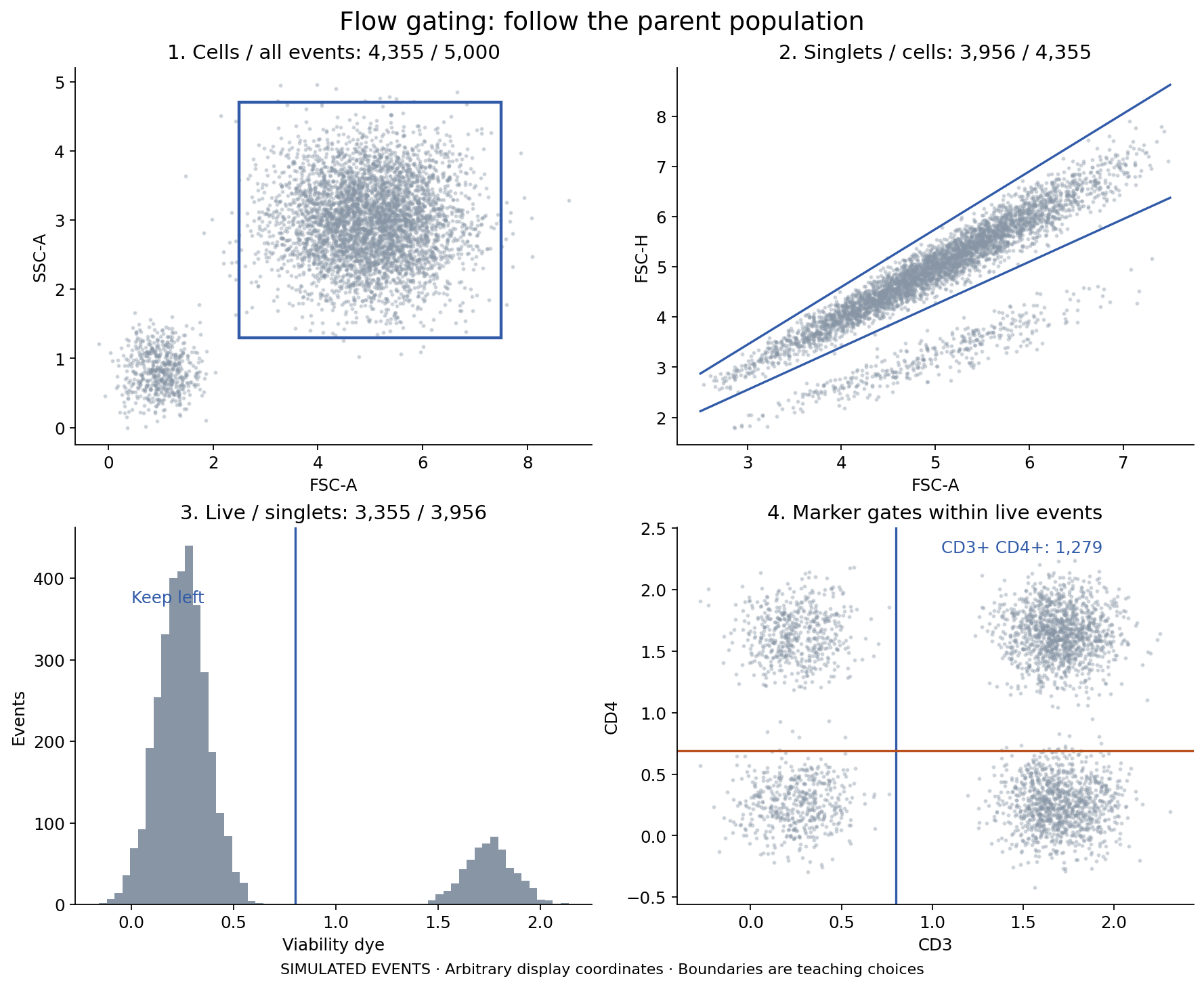
The first panel plots forward-scatter area (FSC-A) against side-scatter area (SSC-A). Our rectangle retains 4,355 of 5,000 events. We call it “Cells” for this example. Scatter alone does not establish a specific lineage or prove that every retained event is a viable cell; that interpretation requires the specimen and marker context.
The downloadable script uses FSC-A from 2.5 to 7.5 and SSC-A from 1.3 to 4.7. Those numbers have no meaning on a real instrument. Review the distribution and experimental controls instead of copying coordinates from a tutorial.
2. Review singlets within that parent
Panel 2 shows FSC-H against FSC-A only for events inside “Cells.” Our simulated singlets lie near a height-to-area ratio of one, and the gate keeps ratios from 0.85 to 1.15. It retains 3,956 events. In an experiment, pulse area, height, or width can help discriminate aggregates; the useful channel combination and boundary depend on the acquired data. [1]
3. Inspect viability within singlets
The viability histogram contains those 3,956 singlet events. Selecting simulated dye values below 0.8 retains 3,355 events. A real viability boundary needs an appropriate dye and controls, interpreted in the context of the staining and fixation procedure. A low-scatter gate is not a substitute for that measurement.
4. Define the marker population
Within “Live,” our illustrative CD3 threshold of 0.8 selects 2,333 events. We then evaluate CD4 only within that CD3-positive parent. The CD4 threshold comes from a separate simulated FMO distribution, described below. This final gate contains 1,279 events.
Although the last plot displays every live event, only its upper-right region contributes to the final CD3-positive, CD4-positive count. Keeping the plot parent and the reported gate parent explicit prevents a common interpretation error.
What an FMO control can tell you
A fluorescence-minus-one (FMO) control contains the other panel stains while omitting the marker being evaluated. It helps characterize background and spreading in that marker’s measurement. An unstained sample, an FMO, a single-stain compensation control, and a biological negative control answer different questions. BD’s controls guide explains why control choice must follow the experiment and the source of background. [2]
For a reproducible teaching boundary, we generated 2,000 FMO-like CD4 display values from a normal distribution with mean 0.25 and standard deviation 0.20. Their 99th percentile is 0.6886, which we use as the CD4 threshold. This retains about 1% of that simulated control above the line by design. It is not a recommendation to use a universal 1% rule, and it does not establish specificity or a false-discovery rate in stained samples.
The simulated positive and negative clouds are deliberately simple. Real controls can show overlapping distributions and sample-dependent backgrounds. Review a proposed threshold against relevant biological controls and representative samples, especially when interpreting dim expression.
The denominator changes the result
| Population | Events | % of parent | % of all events |
|---|---|---|---|
| All events | 5,000 | — | 100.00% |
| Cells | 4,355 | 87.10% | 87.10% |
| Singlets | 3,956 | 90.84% | 79.12% |
| Live | 3,355 | 84.81% | 67.10% |
| CD3+ | 2,333 | 69.54% | 46.66% |
| CD4+ within CD3+ | 1,279 | 54.82% | 25.58% |
The final population is 54.82% of its CD3-positive parent but 25.58% of all acquired events. Both calculations are correct. Reporting only “54.82% CD4 positive” leaves the reader unable to reconstruct what was counted. Use the same parent definition when comparing samples.
Review and report the strategy
Inspect representative samples from each condition before propagating gates. Back-gate a selected population onto earlier plots to see where its events originated. Record adjustments and the reasons for them; a shifted population may require investigating biology or technical quality before moving a boundary.
Preserve the original event files, gate hierarchy, parent populations, channel mapping, compensation or unmixing settings, transforms, and control rationale. MIFlowCyt provides a reporting framework covering the experiment, specimens, instrument, and analysis. These records let another analyst understand what your percentages represent. [3]
Finally, events from one sample are not independent biological replicates. A sample containing thousands of cells still contributes one sample-level population summary unless the experimental design specifies a different unit of analysis.
To apply the workflow in Gradiance, start with the flow cytometry documentation. Open a sample from its workspace and confirm its identity before interpreting the plots. The standalone workbench can show a synthetic demo; the appearance of a gating plot by itself does not establish which data it contains.
Reproduce the hierarchy
- 5,000 simulated events in display coordinates (CSV)
- 2,000 simulated FMO-like CD4 values (CSV)
- Python script for all three teaching examples
- Calculated results and package versions
Install NumPy, SciPy, and Matplotlib in a Python environment, then run python reproduce.py --output generated. The script generates the simulated data, performs the calculations, and draws the figures locally. It does not call Gradiance or submit data to a service. Our recorded versions are NumPy 1.26.4, SciPy 1.17.1, and Matplotlib 3.10.9.
References
- Cossarizza A et al. Guidelines for the use of flow cytometry and cell sorting in immunological studies (third edition). European Journal of Immunology. 2021.
- BD Biosciences. Flow cytometry controls: tips for better data.
- Lee JA et al. MIFlowCyt: the minimum information about a flow cytometry experiment. Cytometry Part A. 2008.