Two parameters from one slope.

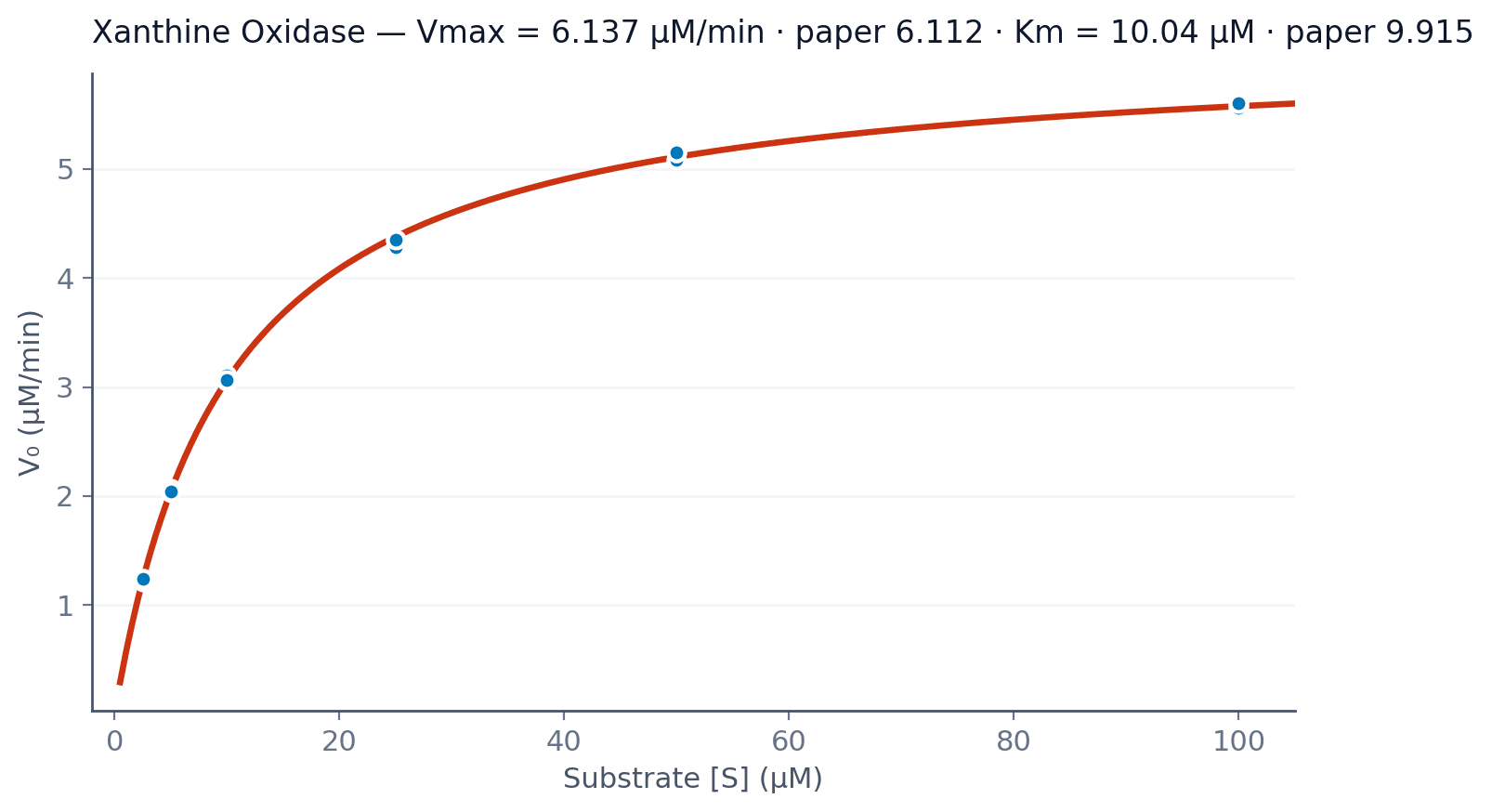
Vmax 6.137 µM/min, Kₘ 10.04 µM, R² = 0.9998. The paper reports 6.112 and 9.915. Six substrate points from 2.5 to 100 µM, xo_kinetics_control.csv in the database — the no-inhibitor arm of a larger study.

Xanthine on xanthine oxidase, no inhibitor. The CSV ships six substrate concentrations — 2.5, 5, 10, 25, 50, 100 µM — at n = 3 replicates each, eighteen rows in total. Initial rates were already computed in the file (slope of the first segment of an absorbance trace at 295 nm), so Gradiance fit Michaelis-Menten directly on (substrate, v₀) without touching the OD.

Vmax is the velocity asymptote at saturating substrate; Kₘ is the substrate concentration at half-Vmax. Vmax came back at 6.137 µM/min against the paper's 6.112, a 0.4 % gap. Kₘ at 10.04 µM against 9.915, a 1.3 % gap. Kₘ is the looser of the two parameters because it's sensitive to where the low-substrate points fall.

Six substrate points is on the lean side for a Michaelis-Menten fit, but the triplicates buy back a lot of degrees of freedom. Three substrates sit below the fitted Kₘ and three above — that's the right shape. If your assay throws everything above 5×Kₘ you fit Vmax fine and pin Kₘ to whatever the optimizer wants. With this range, Kₘ converges cleanly.

Gradiance fits on the untransformed axes — substrate in, velocity out — using nonlinear regression. A Lineweaver-Burk plot is available for figures, but the parameter estimates always come from the original data. The double-reciprocal transform weights low substrate too heavily and is a bad place to fit from, even if it produces a tidier-looking straight line.

import pandas as pd
from scipy.optimize import curve_fit
import numpy as np

def mm(s, vmax, km):
    return vmax * s / (km + s)

# substrate_uM, replicate, v0_uM_per_min  (18 rows: 6 [S] x n=3)
df = pd.read_csv("xo_kinetics_control.csv")
s = df["substrate_uM"].to_numpy()
v = df["v0_uM_per_min"].to_numpy()

# Fit on the raw replicates so each well counts equally toward the
# residuals — averaging first throws away information.
p0 = [v.max(), np.median(s)]
popt, pcov = curve_fit(mm, s, v, p0=p0, maxfev=10_000)

vmax, km = popt
perr = np.sqrt(np.diag(pcov))
print(f"Vmax = {vmax:.4f} +/- {perr[0]:.4f} uM/min")
print(f"Km   = {km:.4f} +/- {perr[1]:.4f} uM")

Two free parameters between Vmax and Kₘ — this fit converges fast and reliably, which makes it the right first step before setting up an inhibition study against the same enzyme.