ΔΔCt without the spreadsheet gymnastics.

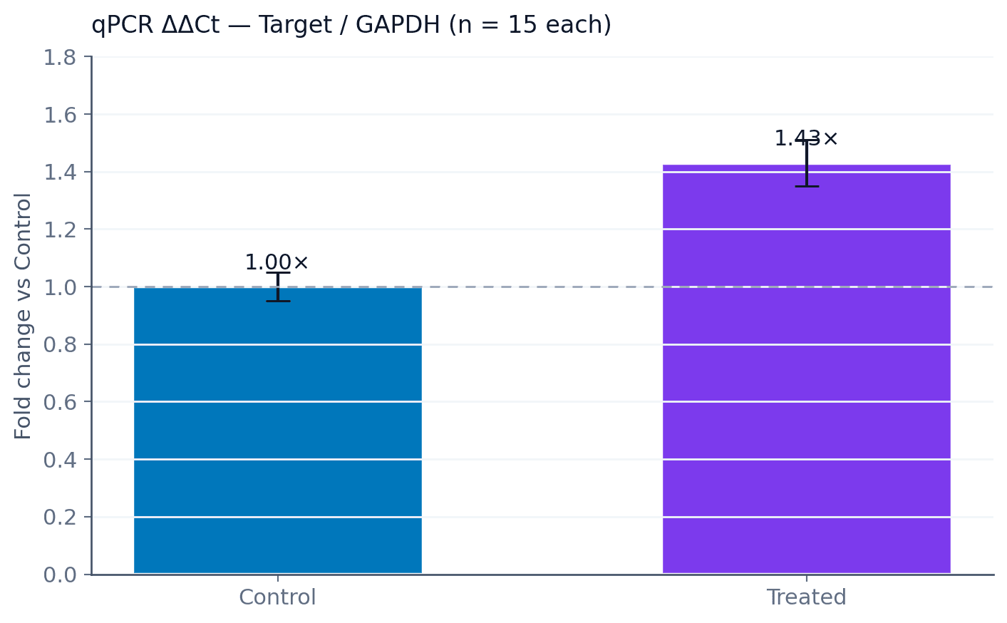
Two conditions, fifteen samples each: control vs. treated, target gene normalised to GAPDH. Treated comes back at 1.43-fold relative to control (ΔΔCt = −0.51). Control is fixed at 1.0× by definition, so the headline is one number — and the audit trail behind it.

The CSV is wide: sample_id, condition, target_ct, reference_ct — one row per sample, target and reference Ct already in their own columns. Gradiance computes the per-sample ΔCt as target minus reference, the ΔΔCt as each sample's ΔCt minus the mean of the control-arm ΔCts, and the fold-change as 2 to the negative ΔΔCt.

Livak and Schmittgen, 2001: fold-change = 2^(−ΔΔCt). The work is in the book-keeping — getting the pivot right, getting the reference assignment right, and computing the right ΔCt mean for the control arm before you subtract it from every well.

The relative method assumes the reference gene is stable across conditions. If you break that silently the fold-changes drift in a way that looks clean on the bar plot. Gradiance computes the CV of the reference Ct across conditions and flags anything above 5 % as a stability warning.

For studies where one reference gene isn't enough — primary tissue, treated cells, anything with a strong stress response — geometric-mean normalisation across two or three references (Vandesompele et al., 2002) is a flag in the new-run picker. The math after that step is identical.

import pandas as pd

# sample_id, condition, target_ct, reference_ct  (n = 30, 15 per arm)
df = pd.read_csv("qpcr_ddct.csv")

df["dCt"] = df["target_ct"] - df["reference_ct"]

mean_ctrl_dct = df.loc[df["condition"] == "Control", "dCt"].mean()  # 4.455
df["ddCt"] = df["dCt"] - mean_ctrl_dct
df["fold_change"] = 2 ** (-df["ddCt"])

summary = (
    df.groupby("condition")["fold_change"]
      .agg(["mean", "std", "count"])
      .reset_index()
)
print(summary)
# Control 1.0000   Treated 1.4267

Two-condition fold-change bars hide the per-sample spread. A 1.43× mean with a 0.3× spread tells a different story from one with a 0.05× spread, but both look the same without error bars. Gradiance always renders the 95 % CI; the export bundle also includes a strip-plot variant with each replicate as a dot, which is the version that paste-into-a-supplementary deserves.